How to access the Normalized digital surface model with stac

from odc import stac as odc_stac
import xarray as xr
import matplotlib.pyplot as plt
import geopandas
import numpy as np
from pystac_client import Client

Connect to the eodc stac

eodc_catalog = Client.open(
    "https://stac.eodc.eu/api/v1",
)

# Select the region
bbox = [16.75, 47.92, 16.79, 47.95]

# Normalized digital surface model (if you want to use the Digital terrain model use collections=["topo-dc-austria-dtm"] and for the Digital surface model use collections=["topo-dc-austria-dsm"])
search = eodc_catalog.search(
    collections=["topo-dc-austria-ndsm"],
    # collections=["topo-dc-austria-dtm"],
    # collections=["topo-dc-austria-dsm"],
    bbox = bbox,
)

print("We found ", search.matched(), " items, that match our filter criteria.")

items = list(search.items())

We found  16  items, that match our filter criteria.

Select all items with the datetime 2024

Even if the time of the data is 2024 the time of the collected data is 2023, so keep that in mind depending on what you want to calculate

items_2024 = []
for item in items:
    dt = item.properties.get("datetime", "")
    if dt.startswith("2024"):
        items_2024.append(item)

items_2024

[<Item id=N2785312_E4827535_nDSM_2024>,
 <Item id=N2785312_E4823439_nDSM_2024>,
 <Item id=N2781216_E4827535_nDSM_2024>,
 <Item id=N2781216_E4823439_nDSM_2024>]

Create a xarray dataset from the items

crs = "EPSG:3035"   # native CRS
res = 1             # meters (from gsd)

ds_2024 = odc_stac.load(
    items_2024,
    crs=crs,
    resolution=res,
    bbox=bbox,
)

print(ds_2024)

<xarray.Dataset> Size: 94MB
Dimensions:      (y: 3597, x: 3274, time: 1)
Coordinates:
  * y            (y) float64 29kB 2.783e+06 2.783e+06 ... 2.779e+06 2.779e+06
  * x            (x) float64 26kB 4.825e+06 4.825e+06 ... 4.828e+06 4.828e+06
    spatial_ref  int32 4B 3035
  * time         (time) datetime64[ns] 8B 2024-09-15
Data variables:
    data         (time, y, x) float32 47MB 0.4529 0.1094 0.0 0.0 ... 0.0 0.0 0.0
    mask         (time, y, x) float32 47MB 255.0 255.0 255.0 ... 255.0 255.0

# print some values
ds_2024["data"].isel(time=0, y=slice(0, 5), x=slice(0, 5)).values

array([[4.52926636e-01, 1.09436035e-01, 0.00000000e+00, 0.00000000e+00,
        2.13623047e-04],
       [1.28112793e-01, 2.02941895e-02, 0.00000000e+00, 4.42504883e-04,
        4.27246094e-04],
       [0.00000000e+00, 0.00000000e+00, 3.50952148e-04, 3.35693359e-04,
        4.73022461e-04],
       [1.37329102e-04, 3.05175781e-05, 0.00000000e+00, 4.57763672e-05,
        1.52587891e-04],
       [0.00000000e+00, 0.00000000e+00, 0.00000000e+00, 0.00000000e+00,
        0.00000000e+00]], dtype=float32)

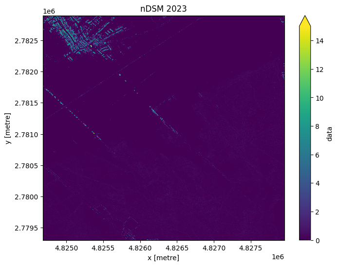
Plot only the data

import matplotlib.pyplot as plt

plt.figure(figsize=(8, 6))
ds_2024["data"].isel(time=0).plot(
    cmap="viridis",
    vmin=0,
    vmax=15
)
plt.title("nDSM 2023")
plt.show()

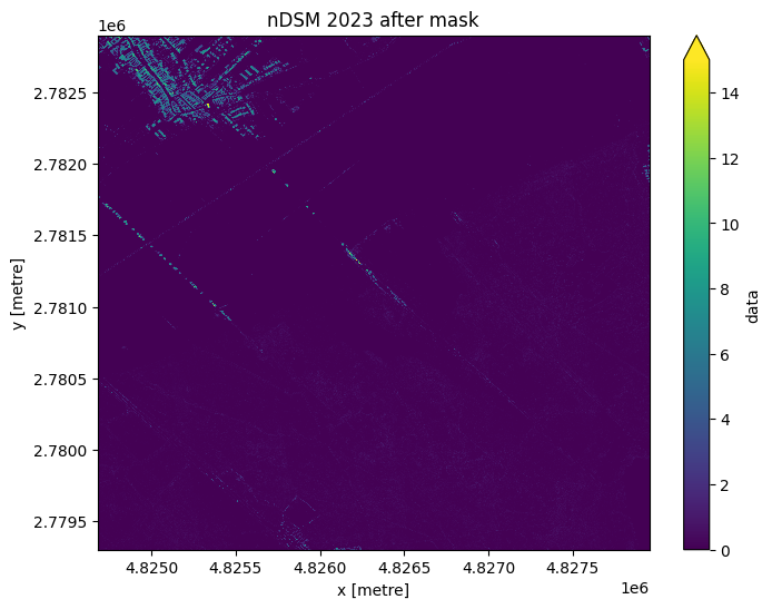
Plot the masked data

da = ds_2024["data"].isel(time=0)
mask = ds_2024["mask"].isel(time=0)

da_masked = da.where(mask == 255)

plt.figure(figsize=(8, 6))
da_masked.plot(
    cmap="viridis",
    vmin=0,
    vmax=15
)
plt.title("nDSM 2023 after mask")
plt.show()

Create a dataset from all years

Sometimes you need to run the stac search again to make it work

crs = "EPSG:3035"   # native CRS -> known from the stac metadata
res = 1             # meters

ds_combined = odc_stac.load(
    items,
    crs=crs,
    resolution=res,
    bbox=bbox,
)

print(ds_combined)

<xarray.Dataset> Size: 377MB
Dimensions:      (y: 3597, x: 3274, time: 4)
Coordinates:
  * y            (y) float64 29kB 2.783e+06 2.783e+06 ... 2.779e+06 2.779e+06
  * x            (x) float64 26kB 4.825e+06 4.825e+06 ... 4.828e+06 4.828e+06
    spatial_ref  int32 4B 3035
  * time         (time) datetime64[ns] 32B 2021-09-15 2022-09-15 ... 2024-09-15
Data variables:
    data         (time, y, x) float32 188MB 0.8824 0.007553 0.0 ... 0.0 0.0 0.0
    mask         (time, y, x) float32 188MB 255.0 255.0 255.0 ... 255.0 255.0

from pyproj import Transformer

lon_min, lat_min, lon_max, lat_max = 16.773838,47.934488,16.773908,47.934538

t = Transformer.from_crs("EPSG:4326", "EPSG:3035", always_xy=True)
x_min, y_min = t.transform(lon_min, lat_min)
x_max, y_max = t.transform(lon_max, lat_max)

# make sure min/max are ordered
x0, x1 = sorted([x_min, x_max])
y0, y1 = sorted([y_min, y_max])

print(x0, y0, x1, y1)

4826606.8683285285 2781068.5887244726 4826611.581265222 2781074.605533941

Create a subset for detailed analysis

subset = ds_combined.sel(
    x=slice(x0, x1),
    y=slice(y1, y0),
)
print(subset)

<xarray.Dataset> Size: 1kB
Dimensions:      (y: 6, x: 5, time: 4)
Coordinates:
  * y            (y) float64 48B 2.781e+06 2.781e+06 ... 2.781e+06 2.781e+06
  * x            (x) float64 40B 4.827e+06 4.827e+06 ... 4.827e+06 4.827e+06
    spatial_ref  int32 4B 3035
  * time         (time) datetime64[ns] 32B 2021-09-15 2022-09-15 ... 2024-09-15
Data variables:
    data         (time, y, x) float32 480B 0.0 0.0005722 ... 0.0003815 0.0005188
    mask         (time, y, x) float32 480B 255.0 255.0 255.0 ... 255.0 255.0

data = subset["data"].where(subset["mask"] == 255)

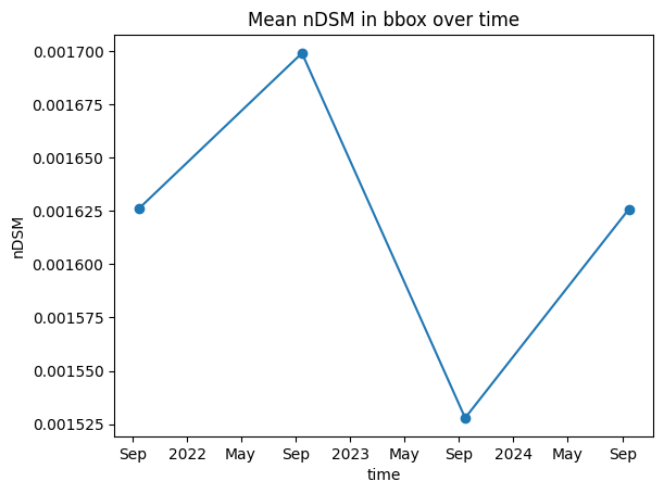
ts_mean = data.mean(dim=("y", "x"))
print(ts_mean.values)

[0.00162608 0.00169907 0.00152791 0.00162582]

ts_mean.plot(marker="o")
plt.title("Mean nDSM in bbox over time")
plt.ylabel("nDSM")
plt.show()

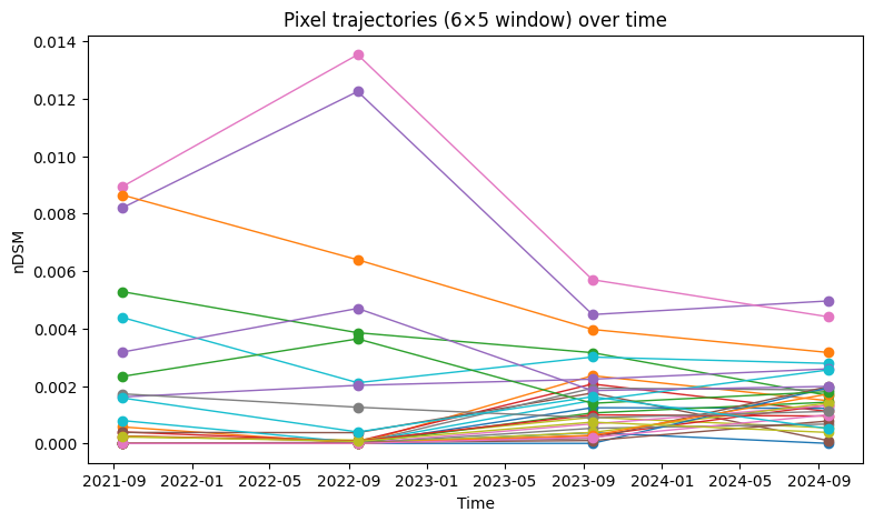
Plot the trajectories of each pixel over the years

sub_data = subset["data"]              # (time, y, x)
pix = sub_data.stack(pixel=("y", "x"))  # (time, pixel)

plt.figure(figsize=(9, 5))
for i in range(pix.sizes["pixel"]):
    plt.plot(pix["time"].values, pix.isel(pixel=i).values, marker="o", linewidth=1)

plt.title("Pixel trajectories (6×5 window) over time")
plt.xlabel("Time")
plt.ylabel("nDSM")
plt.show()