STAC connect to ClimateDT weather stations

from odc import stac as odc_stac
from pystac_client import Client
import xarray as xr
import xarray as xr
import numpy as np

Connect to the eodc stac with pystac CLient

eodc_catalog = Client.open(
    "https://stac.eodc.eu/api/v1",
)

collection = "climatedt"

search = eodc_catalog.search(collections=[collection])
for item in search.items():
    print(item.id)

IFS-NEMO-ScenarioMIP-snowDepth
IFS-NEMO-ScenarioMIP
IFS-FESOM-story-nudging-Tplus2
IFS-FESOM-story-nudging-hist
IFS-FESOM-story-nudging-cont
IFS-NEMO-HighResMIP
IFS-NEMO-CMIP6

item = next(
    eodc_catalog.search(collections=[collection], ids=["IFS-FESOM-story-nudging-Tplus2"]).items()
)
item

• type "Feature"
• stac_version "1.1.0"
• stac_extensions[] 0 items
• id "IFS-FESOM-story-nudging-Tplus2"
• geometry

  • type "Polygon"
  • coordinates[] 1 items

    • 0[] 5 items

      • 0[] 2 items

        • 0 9.47

        • 1 46.34

      • 1[] 2 items

        • 0 17.22

        • 1 46.34

      • 2[] 2 items

        • 0 17.22

        • 1 49.04

      • 3[] 2 items

        • 0 9.47

        • 1 49.04

      • 4[] 2 items

        • 0 9.47

        • 1 46.34
• bbox[] 4 items

  • 0 9.47

  • 1 46.34

  • 2 17.22

  • 3 49.04
• properties

  • title "IFS-FESOM story-nudging Tplus2"
  • description "Model: IFS-FESOM Activity: story-nudging Experiment: Tplus2.0K Resolution: high"
  • end_datetime "2023-12-31T00:00:00Z"
  • start_datetime "2017-01-01T00:00:00Z"
  • datetime None
• links[] 4 items

  • 0

    • rel "collection"
    • href "https://stac.eodc.eu/api/v1/collections/climatedt"
    • type "application/json"

  • 1

    • rel "parent"
    • href "https://stac.eodc.eu/api/v1/collections/climatedt"
    • type "application/json"

  • 2

    • rel "root"
    • href "https://stac.eodc.eu/api/v1"
    • type "application/json"
    • title "EODC Data Catalogue"

  • 3

    • rel "self"
    • href "https://stac.eodc.eu/api/v1/collections/climatedt/items/IFS-FESOM-story-nudging-Tplus2"
    • type "application/geo+json"
• assets

  • data

    • href "https://objects.eodc.eu/68e13833a1624f43ba2cac01376a18af:destine-climate-dt/climate-dt.zarr"
    • type "application/vnd.zarr; version=3"
    • title "IFS-FESOM story-nudging Tplus2"
    • description "Model: IFS-FESOM Activity: story-nudging Experiment: Tplus2.0K Resolution: high"
    • bands[] 2 items

      • 0

        • name "2 metre temperature"
        • description "Near-surface (usually, 2 meter) air temperature"

      • 1

        • name "Total precipitation"
        • description "Represents the amount of water (rain, snow, etc.) as the depth of liquid water if it were all melted and spread evenly."
    • xarray:open_zarr_kwargs

      • group "IFS-FESOM-story-nudging-Tplus2.0K"
      • zarr_format 3
      • consolidated True
    • roles[] 1 items

      • 0 "data"
• collection "climatedt"

asset = item.assets["data"]
store_url = asset.href
print("href:", store_url)

href: https://objects.eodc.eu/68e13833a1624f43ba2cac01376a18af:destine-climate-dt/climate-dt.zarr

Open data with xarray

coords = xr.open_zarr(
    store_url,
    **asset.extra_fields["xarray:open_zarr_kwargs"]
)

print(coords)

<xarray.Dataset> Size: 4GB
Dimensions:    (datetimes: 438288, points: 629)
Coordinates:
  * datetimes  (datetimes) datetime64[ns] 4MB 1990-01-01 ... 2039-12-31T23:00:00
    latitude   (points) float64 5kB dask.array<chunksize=(629,), meta=np.ndarray>
    longitude  (points) float64 5kB dask.array<chunksize=(629,), meta=np.ndarray>
  * points     (points) int64 5kB 0 1 2 3 4 5 6 ... 622 623 624 625 626 627 628
Data variables:
    2t         (datetimes, points) float64 2GB dask.array<chunksize=(438288, 100), meta=np.ndarray>
    tp         (datetimes, points) float64 2GB dask.array<chunksize=(438288, 100), meta=np.ndarray>

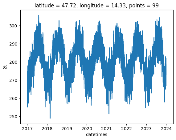
coords["2t"].isel(points=99).plot()

[<matplotlib.lines.Line2D at 0x7d2bae668210>]

Create subset with bbox and year

# Bounding box
lon_min, lat_min, lon_max, lat_max = 15.839539,47.565407,16.877747,48.039529
# Compute lat/lon (small, so this is fast)
lats = coords.latitude.compute()
lons = coords.longitude.compute()

# Boolean mask for points within the bbox
mask = (
    (lats >= lat_min) & (lats <= lat_max) &
    (lons >= lon_min) & (lons <= lon_max)
)

# Subset
ds_subset = coords.sel(points=mask.values)

ds_2023 = ds_subset.sel(datetimes=ds_subset.datetimes.dt.year == 2023).compute()
print(ds_2023)

<xarray.Dataset> Size: 5MB
Dimensions:    (datetimes: 8760, points: 34)
Coordinates:
  * datetimes  (datetimes) datetime64[ns] 70kB 2023-01-01 ... 2023-12-31T23:0...
    latitude   (points) float64 272B 48.01 48.01 47.85 ... 47.6 47.58 47.74
    longitude  (points) float64 272B 16.84 16.24 16.54 ... 16.29 16.1 16.39
  * points     (points) int64 272B 0 5 22 31 33 60 ... 332 377 378 381 382 383
Data variables:
    2t         (datetimes, points) float64 2MB 279.0 276.1 276.1 ... 274.2 273.0
    tp         (datetimes, points) float64 2MB 0.0 0.0 0.0 ... 0.0 2.936e-06 0.0

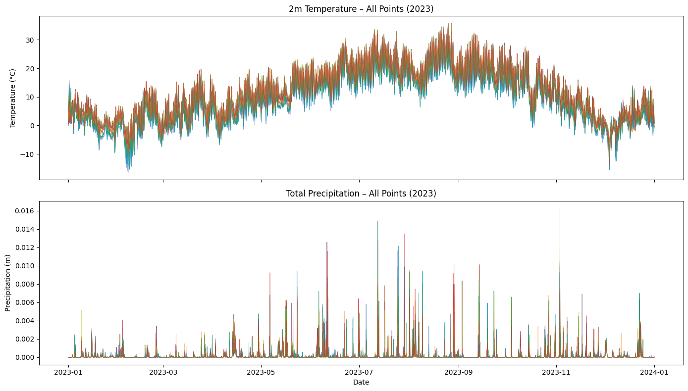
Plot both values over 2023

import matplotlib.pyplot as plt

# Select 2024 and compute

# --- Plot 2t (2m Temperature) ---
fig, axes = plt.subplots(2, 1, figsize=(14, 8), sharex=True)

for point in ds_2023.points.values:
    axes[0].plot(
        ds_2023.datetimes,
        ds_2023["2t"].sel(points=point) - 273.15,  # K to °C
        alpha=0.5, linewidth=0.7
    )
axes[0].set_title("2m Temperature – All Points (2023)")
axes[0].set_ylabel("Temperature (°C)")

# --- Plot tp (Total Precipitation) ---
for point in ds_2023.points.values:
    axes[1].plot(
        ds_2023.datetimes,
        ds_2023["tp"].sel(points=point),
        alpha=0.5, linewidth=0.7
    )
axes[1].set_title("Total Precipitation – All Points (2023)")
axes[1].set_ylabel("Precipitation (m)")

plt.xlabel("Date")
plt.tight_layout()
plt.show()