EODC Dask Tutorial¶

Dask is a flexible parallel computing library for analytics that enables you to scale your computations from a single machine to a cluster. This tutorial will guide you through the basics of using Dask on the EODC cluster. The computation will take place on the cluster and you only need to download the result to your local machine for visualisation or further processing steps. As input data for this tutorial we will use output data from the Global Flood Monitoring (GFM) service.

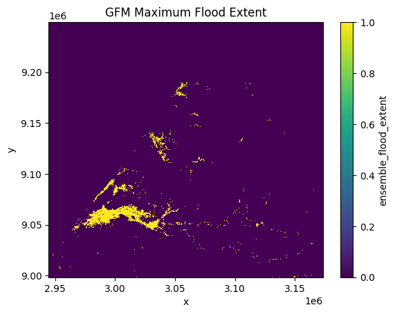
As an example, we will calculate the maximum flood extent of a certain time range over an area of interest in Morocco.

Prerequisites¶

Before we start, make sure you have installed all the necessary Python libraries and packages with the correct versions. It is important that the cluster and client (your machine) have the same versions for the key Python libraries. The easiest way is to create a new Python environment with the package manager of your liking. See the required dependencies in the EODC cluster image repository.

In order to spin up a dedicated cluster on the EODC cluster, you will need to request an EODC account. Please follow the instructions here.

Prepare Python environment¶

In this notebook, we are using Python 3.12.11. First, let’s install some necessary Python packages. We also need to install the “ipykernel” packge to enable Jupyter notebooks to run Python code.

!pip install pyproj xarray shapely pystac_client odc-stac==0.4.0 odc-loader==0.5.1 matplotlib eodc-connect rioxarray ipykernel

!pip install lz4==4.4.4 tornado==6.5.2 toolz==1.0.0 cloudpickle==3.1.1 msgpack==1.1.1

First some imports¶

import pyproj
import rioxarray
import xarray as xr
from pathlib import Path
from datetime import datetime
from shapely.geometry import box
from pystac_client import Client
from odc import stac as odc_stac
import matplotlib.pyplot as plt

from eodc_connect.dask import EODCDaskGateway

Initialize cluster¶

Your username of your EODC account come here, usually it is your email address you have used for registration. After running the next cell, a prompt will open and ask you to enter your password.

your_username = "tobias.raiger-stachl@eodc.eu"
gateway = EODCDaskGateway(username=your_username)

Unclosed client session
client_session: <aiohttp.client.ClientSession object at 0x152462600>

Once authenticated, you can specify the details of your cluster. Specify the number of cores and size of memory of your worker machines. Additionally, you can specify any public docker image which has the same dask version installed like our Dask cluster. However, we suggest you are using our cluster image to avoid errors coming from mismatching software versions.

You will find more detailed information about dask here.

The client object provides you with an URL to the dashboard of your current cluster. Copy/paste this into your web browser to get an overview what is currently happening on your cluster.

Please make sure to re-use or shutdown an existing cluster, before spawning a new one!

# Connect to the gateway and shutdown the existing cluster if it exists
cluster_list = gateway.list_clusters()
if len(cluster_list) > 0:
    gateway.connect(cluster_list[0].name).shutdown()
    print(f"Shutting down {cluster_list[0].name}")
else:
    print("No existing cluster found.")

No existing cluster found.

# Define cluster options
cluster_options = gateway.cluster_options()

# Set the number of cores per worker
cluster_options.worker_cores = 8

# Set the memory per worker (in GB)
cluster_options.worker_memory = 16

# Specify the Docker image to use for the workers
cluster_options.image = "ghcr.io/eodcgmbh/cluster_image:2025.9.3"

# Create a new cluster with the specified options
cluster = gateway.new_cluster(cluster_options)

# Automatically scale the cluster between 1 and 10 workers based on workload
# cluster.adapt(1, 2)  

# Optionally, scale the cluster to use only one worker
cluster.scale(1)

# Get a Dask client for the cluster
client = cluster.get_client()
client.dashboard_link

'https://dask.services.eodc.eu/clusters/dask-gateway.5541687a59e04f27a7d23390720e8494/status'

2026-04-08 15:33:36,587 - distributed.client - ERROR - Failed to reconnect to scheduler after 30.00 seconds, closing client

Search and load data¶

Now we will define our area (AOI) and time range of interest for which we want to calculate the maximum flood extent for.

All GFM data is registered as a STAC collection. Please find more information about STAC in our documentation.

# Define the API URL
api_url = "https://stac.eodc.eu/api/v1"

# Define the STAC collection ID
collection_id = "GFM"

# Define the area of interest (AOI) as a bounding box
# Use portal.gfm.eodc.eu to create an AOI and retrieve the coordinates or another tool like bboxfinder.com
# aoi = box(min_lon, min_lat, max_lon, max_lat)
aoi = box(-6.725286048,34.093280072,-4.792626025,36.073018993)

# Define the time range for the search
time_range = (datetime(2026, 2, 1), datetime(2026, 3, 1))

# Open the STAC catalog using the specified API URL
eodc_catalog = Client.open(api_url)

# Perform a search in the catalog with the specified parameters
search = eodc_catalog.search(
    max_items=1000,             # Maximum number of items to return
    collections=collection_id,  # The collection to search within
    intersects=aoi,             # The area of interest
    datetime=time_range         # The time range for the search
)

# Collect the found items into an item collection
items = search.item_collection()

print(f"On EODC we found {len(items)} items for the given search query")

On EODC we found 187 items for the given search query

We will use the retrieved STAC items to lazily load the data into an xarray.Dataset object. To accomplish this, we need to specify the bands to load, the coordinate reference system (CRS), and the data resolution. All necessary metadata is contained within each STAC item.

There is no strict rule for determining the optimal chunk size, but a general guideline is to set the chunk size as a multiple of the raster file block size that will be read. Additionally, the chunk size should ideally be around 100-300 MB, depending on the available memory on the worker node. The following cell provides an overview of the total array size and estimated chunk size.

In our specific case, the raster block size is 512x512 pixels and the worker has substantial memory capacity. Therefore, we will set the chunk size to 4096x4096 pixels and utilize all available timestamps (-1).

If the processing on the worker node fails, please try reducing the chunk size to e. g. 1024x1024px.

# Extract the coordinate reference system (CRS) from the first item's properties
crs = pyproj.CRS.from_wkt(items[0].properties["proj:wkt2"])

# Set the resolution of the data
resolution = items[0].properties['gsd']

# Specify the bands to load
bands = ["ensemble_flood_extent"]

# Load the data using odc-stac with the specified parameters
xx = odc_stac.load(
    items, 
    bbox=aoi.bounds,   # Define the bounding box for the area of interest
    crs=crs,   # Set the coordinate reference system
    bands=bands,   # Specify the bands to load
    resolution=resolution,   # Set the resolution of the data
    dtype='uint8',   # Define the data type
    chunks={"x": 4096, "y": 4096, "time": -1},  # Set the chunk size for Dask
    dask_client=client,
    groupby="solar_day"
)

# Extract the 'ensemble_flood_extent' data from the loaded dataset
data = xx.ensemble_flood_extent
data

<xarray.DataArray 'ensemble_flood_extent' (time: 22, y: 12534, x: 11448)> Size: 3GB
dask.array<ensemble_flood_extent, shape=(22, 12534, 11448), dtype=uint8, chunksize=(22, 4096, 4096), chunktype=numpy.ndarray>
Coordinates:
  * time         (time) datetime64[us] 176B 2026-02-01T18:32:49 ... 2026-02-2...
  * y            (y) float64 100kB 9.249e+06 9.249e+06 ... 8.998e+06 8.998e+06
  * x            (x) float64 92kB 2.944e+06 2.944e+06 ... 3.173e+06 3.173e+06
    spatial_ref  int32 4B 0
Attributes:
    nodata:   255

Process on the cluster¶

First, we filter the data to exclude invalid values and calculate the sum along the time dimension. The maximum flood extent refers to the largest area covered by flooded pixels during the specified time range. Therefore, we convert the result to a binary mask where each pixel is set to 1 if it was flooded during the specified time range, and 0 if it was not. Then we start the computation on the cluster and save the result as a compressed TIFF file. This file can be visualized in e.g. QGIS.

# Create output directory
output = Path("./output")
output.mkdir(exist_ok=True)
fname = "max_flood_morocco_202602_dask.tif"

# Filter the data to exclude values of 255 (nodata) and 0 (no-flood), then sum
# along the "time" dimension 
filtered_data = data.where((data != 255) & (data != 0))
result = filtered_data.sum(dim="time")

# Convert the result to binary (1 where the sum is greater than 0, otherwise 0)
# and set the data type to uint8 
binary_result = xr.where(result > 0, 1, 0).astype("uint8")

# Compute
computed_result = binary_result.compute()

# 4. Save with specific block sizes and LZW compression
output_path = output.joinpath(fname)
computed_result = computed_result.rio.write_crs(crs)
computed_result.rio.write_nodata(255, inplace=True)
computed_result.rio.to_raster(
    output_path,
    crs=crs,
    compress="LZW",
    tiled=True,
    blockxsize=512,
    blockysize=512
)

Also, we can plot a part of the result with the plotting library matplotlib.

plt.figure()
computed_result[:, :].plot()
plt.title("GFM Maximum Flood Extent")
plt.show()

../_images/67e2baba6814c5707571a82e5be9d5951780fdfa0a0ab53507516cacaec4083a.png

Shutdown cluster¶

After successful processing, we need to shutdown our cluster to free up resources.

# Connect to the gateway and shutdown the existing cluster if it exists
cluster_list = gateway.list_clusters()
if len(cluster_list) > 0:
    gateway.connect(cluster_list[0].name).shutdown()
    print(f"Shutting down {cluster_list[0].name}")
else:
    print("No existing cluster found.")

Shutting down dask-gateway.5541687a59e04f27a7d23390720e8494